3.1 Causal Thinking
Imagine the following scenario. You’re assisting a colleague from the marketing team, and they say:
“The marketing team sent coupons to some users, and their purchase rate was twice as high as those who didn’t receive them. So, the coupons must have doubled the purchase rate!”

Would you agree with this conclusion? At first, it sounds reasonable. But what if you found out the marketing team sent coupons only to customers who had just browsed the product page, added items to their cart, or showed other signs they were ready to buy?
That should raise a red flag. These customers were already more likely to buy, with or without the coupon.
Selection Bias
The real question is: what did the coupons actually change? If we send coupons based on specific criteria, we can’t fairly compare purchase rates. The people who got coupons might have bought anyway, since they were already more engaged.
Selection Bias
The distortion of a causal effect due to non-random assignment of participants, which leads to comparing groups that are not truly comparable.
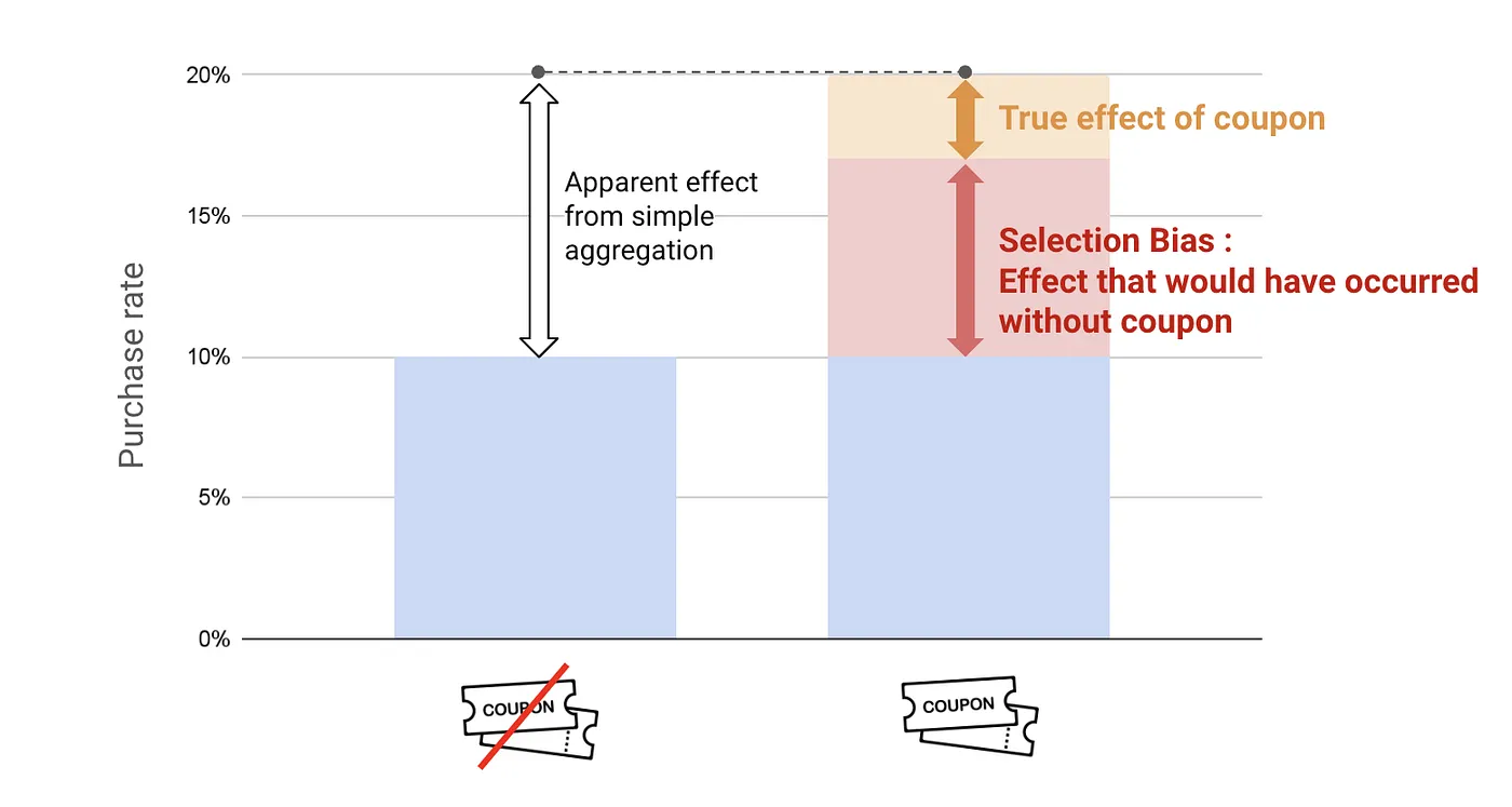
The 10-point gap between groups looks impressive, but most of it was already there before the coupons went out. The real lift from the coupon—the part that wouldn’t have happened otherwise—might be just a few points. The rest is selection bias: the coupon went to people who were likely to buy anyway.
You see this pattern all the time in marketing. Retargeting campaigns show high conversion rates, but that’s because they reach people who already visited your site. Email campaigns look great on revenue per recipient, but those emails go to your most engaged subscribers. In both cases, the treatment and the outcome are linked because of customer intent, not because the treatment caused the outcome.
The Counterfactual
This leads to the key question: what would have happened if we hadn’t done anything?
The main challenge in causal inference is that we only get to see one outcome for each person. If we had a time machine, we could give a customer a coupon, rewind, and see what happens if we didn’t. But in reality, we only see one version of the story for each customer.
Counterfactual
The hypothetical outcome that we cannot observe for the same individual. The treatment effect is the difference between what would happen under treatment and what would happen under control.

Formalizing this makes the problem precise. The treatment effect for a customer is:
\[\tau = Y(1) - Y(0)\]
Here, \(Y(1)\) is what happens if someone gets the treatment, and \(Y(0)\) is what happens if they don’t. The problem is, we only ever see one of these for each person. If we just compare treated and untreated groups without accounting for this, we mix up the true effect with differences that were already there. That’s selection bias.
Simpson’s Paradox
You might think, “If confounders are the problem, I’ll just look at the overall data more carefully.” But confounders can produce wildly misleading results, even reversing the direction of an effect.
Consider a classic example from Judea Pearl’s The Book of Why. Imagine a graph with exercise amount on the x-axis and cholesterol levels on the y-axis. At first glance, the data seems to show that people who exercise more actually have higher cholesterol levels. But that doesn’t make sense!
What’s missing? Age. If you break down the data by age group, you see a different story: within each group, people who exercise more usually have lower cholesterol. The overall trend reversed because older people both exercise more and have higher cholesterol. When you combine the groups, age acts as a confounder.
Simpson’s Paradox
A phenomenon where a trend appears in different groups of data but reverses or disappears when these groups are combined.

This shows up frequently in marketing data. A channel might look unprofitable in aggregate but perform well within specific customer segments, or vice versa. The lesson: always ask whether there is a confounding variable hiding behind the numbers.
Why Not Just Run an A/B Test?
You might wonder, “Why not just run an A/B test?”
In causal inference, A/B testing is known as a Randomized Controlled Trial (RCT) and is often considered the “gold standard” for answering causal questions. By randomly assigning customers to treatment and control groups, we ensure that other factors (such as customer preferences or behavior) are balanced across both groups, which eliminates the bias that would otherwise distort the comparison.
Randomized Controlled Trial (RCT)
An experimental method where participants are randomly assigned to groups to test the effect of an intervention. Because the assignment is random, any difference in outcomes can be attributed to the treatment rather than pre-existing differences.
So if we understand RCTs, does that mean they’re always the perfect solution? Unfortunately, no. While RCTs are the strongest evidence available, there are many situations where they just aren’t feasible:
Opportunity loss. If you run an RCT, half your customers might not get the new product or offer. That could mean missing out on sales, which isn’t always acceptable for the business.
Time constraints. RCTs can be time-consuming. They often require weeks or even months to gather enough data to draw reliable conclusions. Time is money, after all!
Stakeholder complexity. RCTs become even more complex when multiple stakeholders are involved. Not every client or partner has the resources or ability to execute an RCT effectively.
That’s why the rest of this section focuses on tools for measuring causal effects when you can’t run an RCT, and for figuring out who actually benefits when you can.
Road Map for Part 3
Here’s the plan. If you can randomize, A/B testing gives you the most reliable answers—but it’s easy to make mistakes. If you can’t randomize, quasi-experimental methods use natural variation to get as close as possible to what an experiment would show. Once you have a causal estimate, meta-learners and uplift modeling help you see which customers actually respond, so you can avoid spending on people who would have converted anyway.
The next chapter starts with A/B testing, the gold standard. But even the gold standard has pitfalls that can lead you to the wrong answer.