6.2 Building and Optimizing an MMM
What Is Media Mix Modeling?
Media Mix Modeling (MMM) is a statistical approach that uses aggregated time-series data — typically weekly sales and media spend by channel — to estimate how much each marketing channel contributes to business outcomes. Unlike user-level attribution, MMM works with aggregate data and does not require individual tracking, which makes it resilient to cookie loss, App Tracking Transparency, and walled-garden restrictions.
MMM serves three purposes:
- Measure: quantify each channel’s contribution and return on investment (ROI).
- Simulate: answer “what if” questions — what happens to sales if we cut TV spend by 30%?
- Optimize: allocate a fixed budget across channels to maximize the expected outcome.
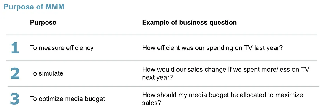
The renewed interest in MMM is not just nostalgia. As user-level tracking becomes less reliable, aggregate modeling is now the most practical way to measure cross-channel media effectiveness.
The MMM Equation
At its simplest, MMM is a regression of weekly sales on media spend, controlling for holidays, promotions, and other non-media drivers:
\[ y_t = \beta_0 + \sum_{c=1}^{C} \beta_c \cdot x_{c,t} + \sum_{k} \gamma_k \cdot z_{k,t} + \varepsilon_t \]
where \(y_t\) is sales at time \(t\), \(x_{c,t}\) is spend in channel \(c\), \(z_{k,t}\) are control variables, and \(\varepsilon_t\) is noise.
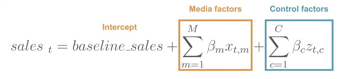
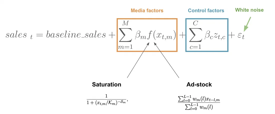
This simple regression is not enough for two reasons. First, media effects are not immediate — a TV ad this week can still influence purchases in the following weeks (carryover). Second, media effects are not linear — the hundredth GRP in a week adds less than the first (diminishing returns).
A more realistic model applies adstock (carryover) and saturation (diminishing returns) transforms before the linear combination:
\[ y_t = \beta_0 + \sum_{c=1}^{C} \beta_c \cdot \text{Saturation}\bigl(\text{Adstock}(x_{c,t})\bigr) + \sum_{k} \gamma_k \cdot z_{k,t} + \varepsilon_t \]
Saturation (Diminishing Returns)
Every media channel eventually saturates. The first million dollars of TV spend drives significant incremental sales; the tenth million drives far less. The Hill function is the most common way to model this:
\[ \text{Hill}(x) = \frac{x^S}{x^S + K^S} \]
where \(K\) (the half-saturation point, often called EC50) is the spend level at which the channel reaches 50% of its maximum effect, and \(S\) (the slope) controls how sharply the curve bends.

The practical takeaway is clear: if Channel A is already saturated and Channel B is still on the steep part of its curve, shifting budget from A to B can increase total return — even if Channel A’s average ROI looks higher.
Adstock (Carryover Effects)
Advertising does not stop working the moment it stops airing. Adstock captures this lagged effect. The simplest form is geometric decay:
\[ \text{Adstock}_t = x_t + \lambda \cdot \text{Adstock}_{t-1} \]
where \(\lambda \in [0, 1]\) is the retention rate. A higher \(\lambda\) means longer carryover. In practice, TV typically shows retention rates around 0.7–0.8 (effects linger for weeks), while digital channels like paid search show rates around 0.3–0.5 (effects decay within days).
More flexible alternatives exist. The Weibull adstock allows the decay shape to be non-monotonic: the effect can peak a few days after exposure before decaying, which better captures channels like email or direct mail where there is a natural processing delay.
Data Requirements
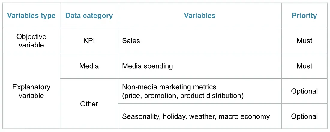
MMM requires three categories of input data:
- Target variable: weekly revenue or sales volume at the brand or product level.
- Media spend: weekly spend per channel (TV, social, display, search, direct mail, etc.).
- Control variables: holidays, seasonality indicators, promotions, pricing changes, competitor activity, macroeconomic factors, or any non-media driver that might explain sales variation.
Recommended granularity:
- Time: Weekly. Daily data is noisier; monthly data has too few observations.
- History: At least 2–3 years of data (about 104 weeks). With less history, it becomes hard to separate media effects from seasonality.
- Geography: National or brand-level is typical. Sub-national (geo-level) models can be more powerful, but they need more data and careful modeling.
- Channels: Only include channels where spend actually varies. If a channel spends the same amount every week, the model cannot learn its effect.
The Bayesian Angle
Before walking through an implementation, one design choice deserves attention: modern MMM is predominantly Bayesian. The reason is practical, not philosophical.
- Priors encode domain knowledge. If your team knows from past experiments that TV ROI is roughly 2.0, you can encode that as a prior. The model updates this belief with the data. Without priors, the model might produce implausible estimates simply because of multicollinearity.
- Credible intervals, not point estimates. Instead of “TV ROI = 2.3,” you get “TV ROI: median 2.3, 90% CI [1.1, 3.8].” A wide interval means you should be cautious about large budget shifts based on that estimate.
- Natural integration with experiments. When you run a geo-lift experiment and estimate a channel’s incremental effect, you can feed that directly into the MMM as an informative prior. This tightens the posterior and improves identifiability — a workflow we develop in detail in Section 6.3.
That’s why tools like Meridian and PyMC-Marketing use Bayesian inference under the hood.
A Walkthrough with Meridian
The companion notebook demonstrates a complete MMM workflow using Google’s Meridian library.
mmm_end_to_end_demo.ipynb — Open in Colab · nbviewer
Committed with outputs; Colab is best-effort. Full list on the Notebooks & Code page.
Meridian is Google’s actively maintained MMM library, the successor to the now-deprecated LightweightMMM. Other strong alternatives include Meta’s Robyn and PyMC-Marketing. The core concepts (adstock, saturation, Bayesian estimation, and budget optimization) are the same across all of these tools. We use Meridian here because it offers a mature API with built-in diagnostics and optimization.
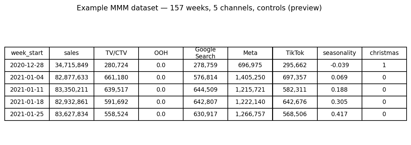
Data loading and preparation. The demo dataset contains 157 weeks of sales data with 5 media channels (TV/CTV, OOH, Google Search, Meta, TikTok) and holiday/seasonality controls. Meridian uses a DataFrameInputDataBuilder to construct its input data from a pandas DataFrame. Scaling is handled internally; no manual normalization is needed. The important detail is that Meridian applies saturation to media_cols (exposure volume such as impressions or clicks), while media_spend_cols are used as the cost basis for ROI.
channels = ["TV/CTV", "OOH", "Google Search", "Meta", "TikTok"]
media_cols = [
    "tv_ctv_impressions", "ooh_impressions", "google_clicks",
    "meta_impressions", "tiktok_impressions",
]
media_spend_cols = [
    "tv_ctv_spend", "ooh_spend", "google_spend",
    "meta_spend", "tiktok_spend",
]
control_cols = [
    "seas_sin52", "seas_cos52",
    "hldy_thanksgiving", "hldy_christmas",
    "trend", "trend_sq",
]

builder = data_frame_input_data_builder.DataFrameInputDataBuilder(
    kpi_type='revenue',
    default_kpi_column='sales',
    default_time_column='time',
    default_geo_column='geo',
)

data = (
    builder
    .with_kpi(df)
    .with_media(df,
        media_cols=media_cols,
        media_spend_cols=media_spend_cols,
        media_channels=channels)
    .with_controls(df, control_cols=control_cols)
    .build()
)
Model training. Meridian uses the No-U-Turn Sampler (NUTS) for MCMC. We first draw from the prior for sanity checks, then sample the posterior.
mmm = model.Meridian(input_data=data, model_spec=model_spec)
mmm.sample_prior(500)
mmm.sample_posterior(
    n_chains=4, n_adapt=500, n_burnin=500, n_keep=1000, seed=SEED
)
# Production runs typically use n_chains=10, n_keep=2000 (≈ 5× compute).
Diagnostics. Meridian’s ModelReviewer runs automated quality checks (convergence, baseline validation, goodness of fit, and prior-posterior shift) and reports a pass/review/fail status.
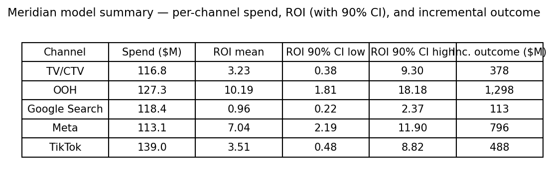
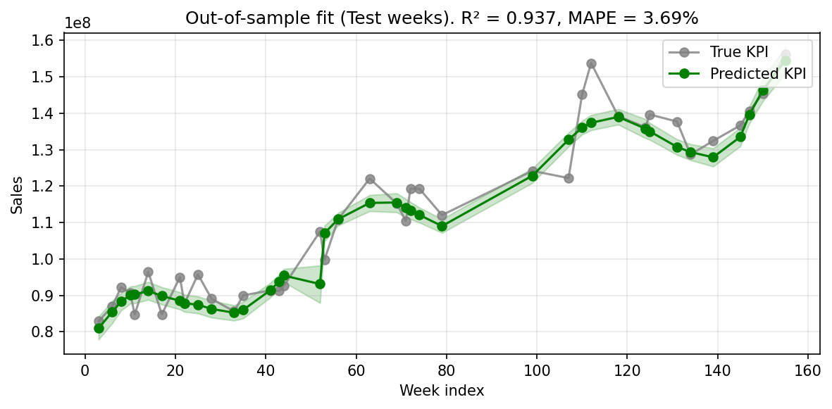
Model fit. With a random 25% week-level holdout, the demo recovers in-sample R² ≈ 0.95 and out-of-sample R² ≈ 0.94. A tight in/out gap is expected here — synthetic data plus a random (interpolation) holdout is close to a best case. On production data with real noise, broken-trend periods, and lumpy promotional activity, out-of-sample R² in the 0.6 to 0.7 range is typical and acceptable. Trust the direction of the media estimates, not just the headline fit.
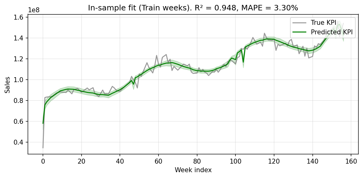
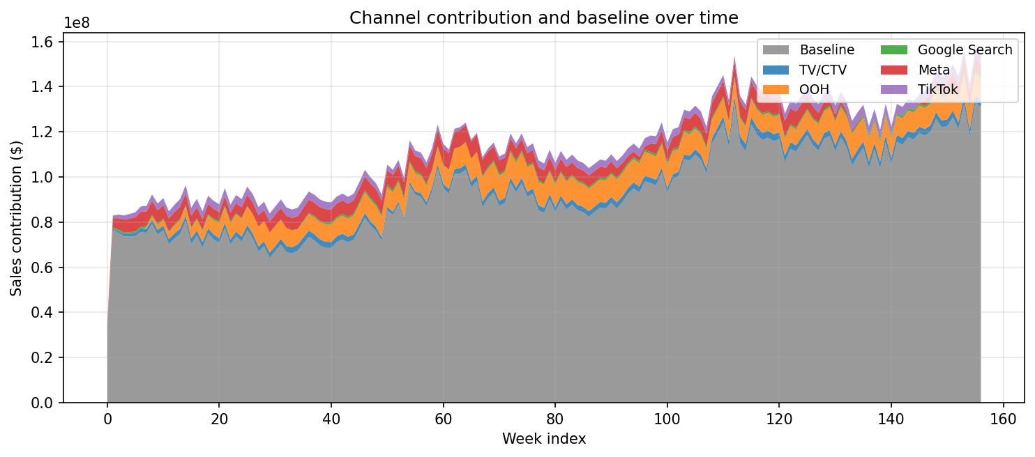
Media insights. The model gives ROI estimates with credible intervals for each channel. Wide intervals mean there is real uncertainty — this is a feature, not a bug. Point estimates alone can be misleading; credible intervals show how much confidence you should have in the results.

Budget Allocation
The model’s three purposes — measure, simulate, optimize — converge here. Once the response curves are fitted, the optimizer searches for the allocation that maximizes predicted KPI under a fixed budget constraint:
budget_optimizer = optimizer.BudgetOptimizer(mmm)
optimization_results = budget_optimizer.optimize()
The intuition is straightforward. If one channel is already saturated and another is still on the steep part of its response curve, shifting dollars from the saturated channel to the unsaturated one increases total predicted sales — even if the saturated channel’s average ROI is higher.
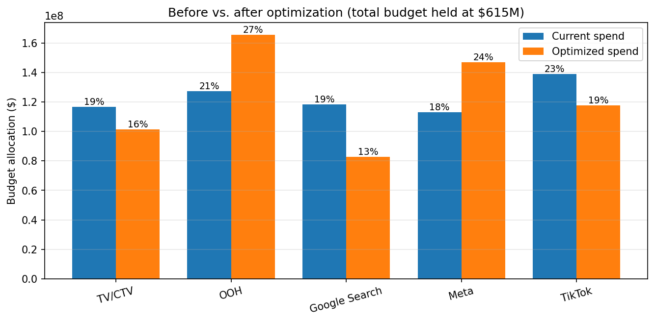
In the demo, the optimizer reallocates spend across the five modeled channels (TV/CTV, OOH, Google Search, Meta, and TikTok), moving budget away from channels with flatter marginal response curves toward channels with more remaining headroom. The total budget stays the same — only the mix changes. Gains of 5–10% in predicted sales from reallocation alone are common when teams first implement MMM; this demo shows about +7%.
Treat the optimizer’s output as a principled starting point, not a finished media plan. The optimizer does not know about contractual commitments, minimum channel presence, operational lead times, or seasonality — those constraints need to come from outside the model. And since the response curves are based on observational data, the next step is to anchor them with experimental evidence. That’s the focus of Section 6.3.
Key Takeaways
- MMM estimates channel contribution using aggregate data. It does not need user-level tracking, so it is resilient to cookie deprecation, App Tracking Transparency, and walled-garden limits.
- Hill saturation and geometric adstock are the two main transforms. Each channel gets its own set of parameters.
- Optimize based on marginal ROI, not average ROI. A channel with high average ROI might already be deep into its saturation curve. Shifting dollars to a channel that is still on the steep part of its curve can increase total return, even if its average ROI is lower.
- Data requirements are specific: weekly data, at least 2–3 years of history, and real spend variation for each channel.
- Bayesian estimation is now the default. Priors let you encode domain knowledge, and the posterior gives credible intervals instead of just point estimates.