The sales team wants a lower price. They are closest to the customer, and they can see the obvious effect: when price drops, units move.
The finance team wants a higher margin. Looking at the same tradeoff from the other side, they can see that revenue can go up while profit disappears if the extra volume is bought too cheaply.
Marketing sits between these views, but not by averaging them. Its job is to connect customer response, brand position, and commercial objectives: when to chase units or revenue, when to protect margin, and when price itself sends a positioning signal.
Both sides are partly right. Price affects volume, but volume is not always the main goal. Sometimes the business wants revenue, sometimes margin, sometimes traffic or share, or even just to clear inventory or defend a price position. The real missing piece is not the objective. It is understanding how much volume actually changes when price moves.
That is what price elasticity gives us. It does not decide the business goal. It gives the response curve that lets us compare pricing decisions against the goal, whether that goal is units, revenue, margin, or positioning.
What Is Price Elasticity?
Imagine you are deciding whether to raise the price of a top-selling cereal by 10%. Will you lose 5% of units, or 20%? That difference decides whether the price change improves sales, revenue, or margin, or whether it simply pushes shoppers away.
Price elasticity of demand measures the sensitivity of quantity sold to a change in price:
For normal goods, elasticity is negative: raise the price, sell fewer units. For simplicity, we usually talk about the absolute value.
\(|\varepsilon| = 1.6\): a 10% price increase loses 16% of units. Demand is elastic. Price increases are risky because volume falls faster than price rises.
\(|\varepsilon| = 0.5\): a 10% price increase loses only 5% of units. Demand is inelastic. The product has pricing power, and a price increase can lift revenue. If unit costs are stable and known, it may also improve contribution margin.
The same elasticity estimate can support different pricing questions:
Should we move the price? Elastic demand makes price increases risky. Inelastic demand makes them more attractive.
Which outcome should we optimize? Elasticity plus price and volume lets us compare units and revenue. Add variable cost, and the same curve can be used to compare contribution margin.
Data Requirements for Price Elasticity
To estimate price elasticity, you need sales data with real price variation. Typical sources are POS scanner data, panel data, or internal online retail records. Use the effective price—revenue divided by units sold—instead of the shelf price:
Effective price captures discounts, multi-buy offers, and midweek price changes more reliably than the listed price.
Two design choices set the foundation: the time grain and the product grain. Weekly is usually the best time grain because daily data is often noisy, while monthly data can hide price changes inside the month. On the product side, start at the SKU level. A single SKU has one package size, one baseline price, and one demand response, so the price signal is easier to read.
Three things to check before fitting anything:
Unit of analysis. Use SKU × week by default. If SKU × week is too sparse, there are two defensible ways to aggregate. Move to SKU × month when price changes are not too frequent and monthly variation is still visible. Or move to SKU group × week by combining truly comparable SKUs, such as color variants, flavor variants, or same-price items with the same shopper role. Do not aggregate just because products share a brand.
Price variation. You need several distinct price points, no single price dominating the history, and enough time to separate price response from noise. As a rough rule, aim for at least three price points, a 10% price spread, and 26 weeks of history.
Distorted demand signals. Stockouts, unusual promotions, holidays, and one-off events can make volume move for reasons unrelated to price. Flag or remove these observations before treating the relationship as a normal price response.
Estimating the Demand Curve
The workhorse model is the constant-elasticity, or power-law, model:
\[
Q = b_0 \times P^{b_1}
\]
where \(Q\) is quantity, \(P\) is price, \(b_0\) is a scale parameter, and \(b_1\) is the elasticity. For normal goods, \(b_1\) is negative. Taking logs gives a linear relationship, \(\log Q = \log b_0 + b_1 \log P\), so \(b_1\) is the slope in log-log space. The model assumes elasticity is constant across the price range. That is a strong assumption, but it is a reasonable starting point for many consumer goods.
Fit the curve in the original, non-log, space with scipy.optimize.curve_fit to avoid the retransformation bias that comes from fitting in log-space and converting back.
The companion notebook also runs a two-pass estimation: fit once on all data, flag observations where actual divided by predicted units falls outside a sensible band, such as 0.3 to 3.0, and refit without them.
Code
# Pass 1: fit on all datapopt_1, _ = curve_fit(power_model, prices, units, p0=p0, maxfev=10000)# Identify outlierspredicted = power_model(prices, *popt_1)ratio = units / predictedmask = (ratio >0.3) & (ratio <3.0)# Pass 2: refit on clean datapopt_2, pcov_2 = curve_fit( power_model, prices[mask], units[mask], p0=popt_1, maxfev=10000)
Promotional spikes are the usual culprit. Include them blindly, and the model treats promotional volume as normal price response, biasing elasticity away from its true value.
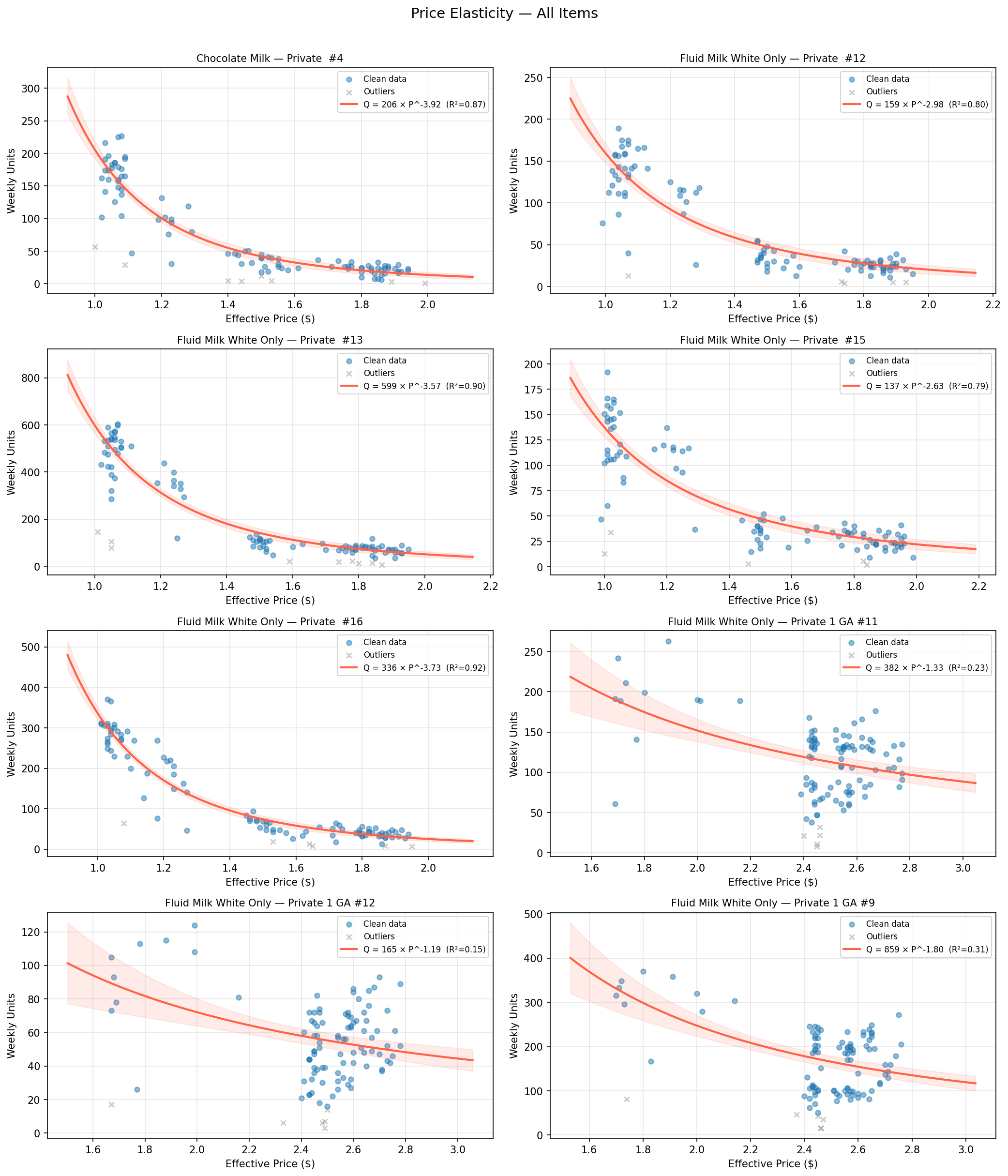
Figure 1: Price–quantity scatter and fitted power curve for a top-selling Fluid Milk SKU (Dunnhumby).
Across the eight top-selling Fluid Milk items, elasticities range from \(-1.2\) for gallon jugs, a staple format with lower elasticity, to \(-3.9\) for smaller formats, which are easier to substitute. Figure 2 shows the fitted curves side by side.
Figure 2: Fitted power-law demand curves for the eight top-selling Fluid Milk products (Dunnhumby).
In practice, an elasticity in the range \(-0.5\) to \(-5\) with \(R^2 > 0.4\) and several distinct price points is usable for pricing decisions. Estimates outside that range are often data problems: too few prices, a single promotional discount dominating the fit, or too short a window. If the elasticity is not believable, neither is any pricing recommendation built on it.
Optimizing for Contribution Margin
Once we have a demand curve, we can ask different pricing questions.
The first is which price maximizes revenue:
\[
\text{Revenue}(P) = P \times Q(P)
\]
This is often the most intuitive starting point because it requires only price and units. If the business does not have reliable variable cost by product or category, revenue may be the practical metric for a first-pass pricing analysis.
But revenue is not profit. If variable cost is available, we can ask the stronger question: which price maximizes contribution margin?
\[
\text{Contribution Margin}(P) = (P - C) \times Q(P)
\]
where \(C\) is variable cost per unit and \(Q(P) = b_0 \times P^{b_1}\).
The two answers can differ. A lower price can sell more units and increase revenue while reducing total margin. A higher price can reduce revenue but improve margin if the remaining units are profitable enough. The point is not that margin is always the only objective. The point is that the objective must be explicit before choosing the price.
Worked example: a private-label cereal
Take a private-label cereal, the same category as the part-introduction promotion story, with these parameters:
Current price: $3.99
Variable cost: $2.20
Current units: 1,500 per week
Estimated elasticity: \(b_1 = -1.6\)
Price
Units
Revenue
Margin per Unit
Total Margin
$3.59 (10% lower)
1,776
$6,376
$1.39
$2,469
$3.99 (current)
1,500
$5,985
$1.79
$2,685
$4.39 (10% higher)
1,288
$5,654
$2.19
$2,821
$4.79 (20% higher)
1,121
$5,369
$2.59
$2,903
The table shows the core tradeoff. Revenue is maximized by cutting the price: the 10% lower price has the highest revenue at $6,376. Margin is maximized by raising the price: the 20% higher price has the highest total margin at $2,903. At 10% higher, revenue falls 5.5% while margin rises 5.1%. Revenue and margin point in opposite directions. This is the discount trap from the part introduction, now with numbers attached.
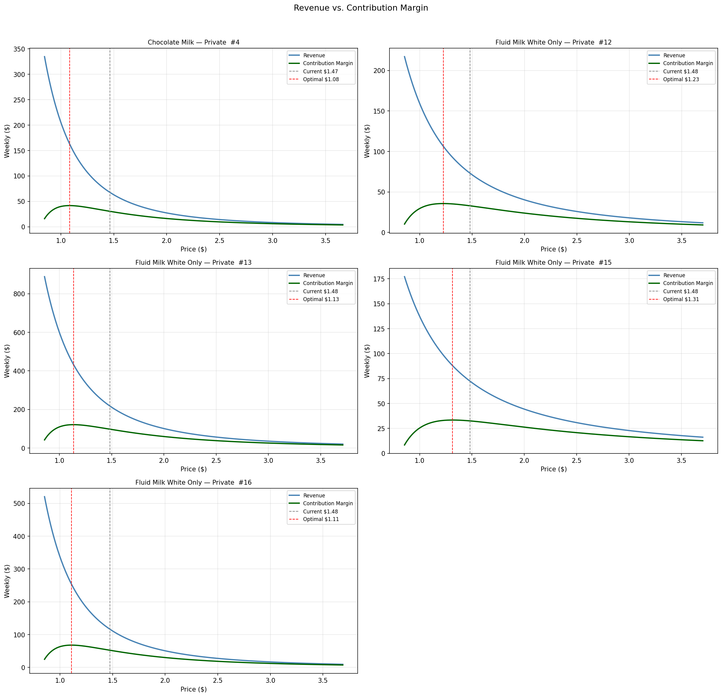
Figure 3 visualizes the same logic for five real Dunnhumby products. In every case, the revenue curve and contribution margin curve peak at different prices. For these highly elastic private-label dairy items, the margin-maximizing price is consistently lower than the current price because the extra volume from a price cut is large enough to lift total margin.
Figure 3: Revenue vs. contribution margin curves for five Fluid Milk products.
The optimization itself is a one-dimensional search. scipy.optimize.minimize_scalar over the negative margin function does the job in a few lines, and the companion notebook walks through it.
Committed with outputs; Colab is best-effort. Full list on the Notebooks & Code page.
Elasticity Varies by Product Role
The same category can contain products with very different shopper roles. In Fluid Milk Products, a gallon of white milk, a single-serve chocolate milk, and a quart of coffee creamer are not interchangeable pricing decisions. They may sit in the same broad commodity, but shoppers buy them for different occasions and compare them against different alternatives.
That is why SKU-level estimates should be aggregated only into comparable SKU groups, such as the same sub-commodity and similar package size. The goal is not to create as many segments as possible. The goal is to avoid averaging together products whose price response should be different.
Figure 4: Units-weighted mean price elasticity by product role within Fluid Milk Products (Dunnhumby).
Before applying one pricing rule across a category, check whether major product roles respond differently. If they do, the average elasticity is not a pricing rule. It is a warning that the category needs to be split more carefully.
Common Pitfalls in Price Elasticity
Endogeneity. Prices are not set at random. If a retailer raises prices during high-demand periods like back-to-school, the observed elasticity is biased toward zero because high prices and high demand co-occur for reasons unrelated to pricing. This is the same selection bias problem from Part 3. Address it with instrumental variables, randomized price experiments, or quasi-experimental designs.
Reference price effects. Customers remember what they paid before. Raising the price usually causes a bigger drop in volume than lowering the price brings in new buyers. The JCPenney “Fair and Square” case is the famous example: switching from promotions to everyday low prices at the same average level led to a sales collapse because customers lost their price anchor.
Competitor reaction. A price cut only works if competitors hold. In concentrated categories, competitors typically match. Everyone sells about the same volume, but at lower margins. Game theory matters more than demand curves there.
Key Takeaways
Price elasticity estimates how much volume changes when price moves. It can support sales, revenue, or margin decisions, depending on the business objective.
Revenue-maximizing and margin-maximizing prices are often different. If reliable variable cost is available, use it to evaluate contribution margin. If not, be explicit that the analysis is optimizing revenue or units, not profit.
SKU × week is the default grain for most retail and online retail elasticity work. If the data is sparse, use SKU × month or carefully constructed SKU groups, but do not mix different price tiers or product roles just to increase sample size.
A single elasticity number can hide large differences across brand tiers, channels, or regions. Check whether major segments respond differently before applying one pricing rule everywhere.
Watch for endogeneity, reference price effects, stockouts, unusual promotions, and competitor reaction. These can make a price response curve look more reliable than it is.
Brodersen, Kay H, Fabian Gallusser, Jim Koehler, Nicolas Remy, and Steven L Scott. 2015. “Inferring Causal Impact Using Bayesian Structural Time-Series Models.”The Annals of Applied Statistics 9 (1): 247–74.
Bult, Jan Roelf, and Tom Wansbeek. 1995. “Optimal Selection for Direct Mail.”Marketing Science 14 (4): 378–94.
Fader, Peter S, Bruce GS Hardie, and Ka Lok Lee. 2005. “Counting Your Customers the Easy Way: An Alternative to the Pareto/NBD Model.”Marketing Science 24 (2): 275–84.
Jin, Yuxue, Yueqing Wang, Yunting Sun, David Chan, and Jim Koehler. 2017. Bayesian Methods for Media Mix Modeling with Carryover and Shape Effects.
Knaflic, Cole Nussbaumer. 2015. Storytelling with Data: A Data Visualization Guide for Business Professionals. Wiley.