3.4 Meta Learners for Treatment Effects
The methods in previous chapters estimate a single number: the Average Treatment Effect (ATE), or the average impact of a treatment across everyone. But in marketing, averages can be misleading. For example, a coupon might increase purchases by 5% on average, but that number hides the real story. Some customers might respond with a 20% lift, while others see no effect or even a drop. If you could identify which customers actually respond, you could spend your budget much more effectively.
Meta-learners try to estimate treatment effects for each individual customer. But what does that actually look like in practice?
Treatment Effects: ATE, CATE, ITE
To define the treatment effect, we turn to the Potential Outcomes Framework. For example, if the potential purchase rate with a coupon is 20% and the purchase rate without the coupon is 10%, the treatment effect is 10%.
Treatment Effect
The difference in outcomes caused by a treatment. Formally: \(\tau = Y(1) - Y(0)\), where \(Y(1)\) is the outcome under treatment and \(Y(0)\) is the outcome under control.

Now, there are three levels of granularity:
- ATE (Average Treatment Effect): the effect averaged across all customers. “Did the coupon increase sales?”
- CATE (Conditional Average Treatment Effect): the average effect for customers with specific characteristics. “Did the coupon work better for urban customers under 30?”
- ITE (Individual Treatment Effect): the effect for a specific individual. Unobservable in practice, but CATE provides our best estimate.
Why does this matter? Because not all customers behave the same way. A price-sensitive customer might jump at a discount, while a brand-loyal customer would have bought at full price anyway. If you know who is who, you can target discounts where they actually drive extra sales, instead of giving away margin to customers who would have purchased regardless.
The Missing Data Problem
Consider this question: did a coupon increase sales? To answer it, we look at data from various customers, including their attributes (age, gender, location), the treatment (coupon or no coupon), and the outcome (purchase or not).
The column \(Y(1)\) represents the outcome when the coupon is used, while \(Y(0)\) represents the outcome without the coupon. If we had both columns for the same individual, calculating the treatment effect would be as simple as subtracting one from the other. But the challenge is that we can only observe one outcome for each individual.
To solve this, we use meta-learners. These are machine learning frameworks that predict what would have happened if a customer had received the other treatment. By filling in these missing counterfactuals, we can estimate the treatment effect for each person.
S-Learner: Start with a Single Model
The “S” in S-learner stands for “Single,” as it relies on a single machine learning model. Train one model on all data with the treatment indicator as an additional feature: \(\hat{Y} = f(X, Z)\). Then estimate CATE by predicting with treatment set to 1 versus 0:
\[\hat{\tau}(x) = \hat{f}(x, 1) - \hat{f}(x, 0)\]
Pseudo-code:
# Train a single model with treatment as a feature
X = df[['age', 'gender', 'location', 'treatment']]
y = df['sales']

model = xgb.XGBRegressor()
model.fit(X, y)

# Predict outcomes under treatment and control
df['sales_treated'] = model.predict(X.assign(treatment=1))
df['sales_control'] = model.predict(X.assign(treatment=0))

# Treatment effect = difference
df['treatment_effect'] = df['sales_treated'] - df['sales_control']
ATE = df['treatment_effect'].mean()
S-learner is the simplest way to start, and often a reasonable baseline. But it has a key weakness: if the treatment effect is small compared to other features, the model can end up ignoring the treatment variable, especially if you use regularization. This means your CATE estimates can be biased toward zero.
T-Learner: Two Separate Models
The “T” in T-learner stands for “Two.” Instead of one model, train separate models for the treated and control groups:
\[\hat{\tau}(x) = \hat{f}_1(x) - \hat{f}_0(x)\]
Pseudo-code:
# Split data into treated and control
df_treated = df[df['treatment'] == 1]
df_control = df[df['treatment'] == 0]

# Train separate models
model_treated = xgb.XGBRegressor()
model_treated.fit(df_treated[['age', 'gender', 'location']], df_treated['sales'])

model_control = xgb.XGBRegressor()
model_control.fit(df_control[['age', 'gender', 'location']], df_control['sales'])

# Predict and subtract
df['sales_treated'] = model_treated.predict(df[['age', 'gender', 'location']])
df['sales_control'] = model_control.predict(df[['age', 'gender', 'location']])

df['treatment_effect'] = df['sales_treated'] - df['sales_control']
ATE = df['treatment_effect'].mean()
T-learner is more flexible because each model can learn different patterns for treated and control groups. But there is a tradeoff: it can have high variance, especially if your treatment and control groups are imbalanced. When you subtract the predictions, errors from both models can add up.
So, S-learner is simple but tends to underestimate effects. T-learner fixes that bias but can be noisy. What can we do next?
Advanced Meta-Learners
Beyond S and T, several more sophisticated methods address their limitations:
- X-Learner: An extension of T-learner designed for imbalanced treatment groups. It imputes the missing counterfactuals and combines them using propensity-score weighting. Works well when one group is much larger than the other.
- DR-Learner (Doubly Robust): Combines outcome modeling and propensity score estimation. Consistent if either model is correctly specified, hence “doubly robust.”
- DML (Double Machine Learning): Uses cross-fitting to avoid overfitting bias, with strong theoretical guarantees. More computationally expensive (~27x slower than S-learner) but provides proper confidence intervals.
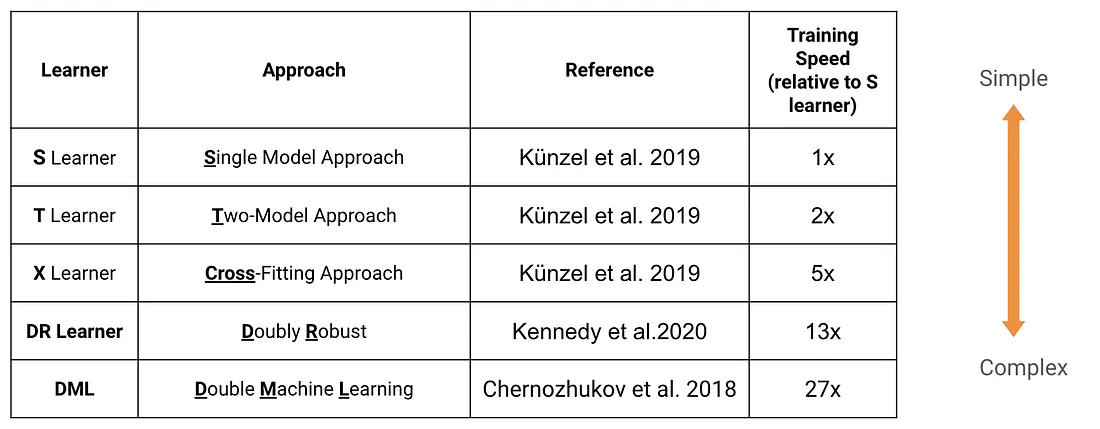
Theory tells us what each method is supposed to optimize. But the real test is seeing how they perform on the same dataset, where you can see the practical differences.
Seeing It in Practice: The Criteo Dataset
We demonstrate meta-learners on the Criteo Uplift dataset, a large-scale advertising RCT released by Criteo AI Lab, containing ~14 million samples with 12 anonymized features. About 85% of users were shown ads (treatment) and 15% were not (control), with a ~0.3% conversion rate.
Since this is a randomized experiment, just comparing conversion rates between treated and control groups gives you an unbiased ATE. The real value of meta-learners here is in showing the differences hidden under that average.
simple_criteo_meta_learners_econml.ipynb — Open in Colab · nbviewer
Committed with outputs; Colab is best-effort. Full list on the Notebooks & Code page.
Most Methods Recover the Average

T-learner and X-learner both match the naive baseline closely, which is what you expect in a randomized experiment with no selection bias. The DML-family estimators (like LinearDML and CausalForestDML) and DR-learner give slightly higher estimates, mostly due to cross-fitting variance, but they are still in the same ballpark. S-learner is not shown in this chart because, when the treatment effect is small compared to the noise, its single model tends to treat the treatment indicator like any other feature. Regularization then shrinks its effect toward zero, so the ATE estimate ends up much lower than the true value. This is a known limitation, not a bug. You can still see S-learner in the CATE distributions and uplift curves, where its narrow spread shows the same bias at the individual level.
